Introduction

This vignette decribes how to solve the mTSP using ompr. The problem is similiar to the standard TSP but now we have more than one Salesman. Please refer to the vignette on the standard TSP for more background information. All salesmen start and end their trips at a single location (the depot). In addition, all salesmen need to visit at least one client.

Setting

First let us import some librarys

library(knitr)
library(dplyr)
library(ggplot2)

The number of cities:

n <- 7

The number of salesmen:

m <- 2

Boundary of our Euclidean space:

# from 0 to ...
max_x <- 500
max_y <- 500

Some random cities and the depot in the middle:

set.seed(1)
cities <- data.frame(id = 1:n, x = c(max_x / 2, runif(n - 1, max = max_x)), 
                                     y = c(max_y / 2, runif(n - 1, max = max_y))) %>% 
  mutate(is_depot = ifelse(id == 1, TRUE, FALSE))
ggplot(cities, aes(x, y)) + 
  geom_point(aes(size = is_depot)) + 
  scale_y_continuous(limits = c(0, max_y)) + 
  scale_x_continuous(limits = c(0, max_x))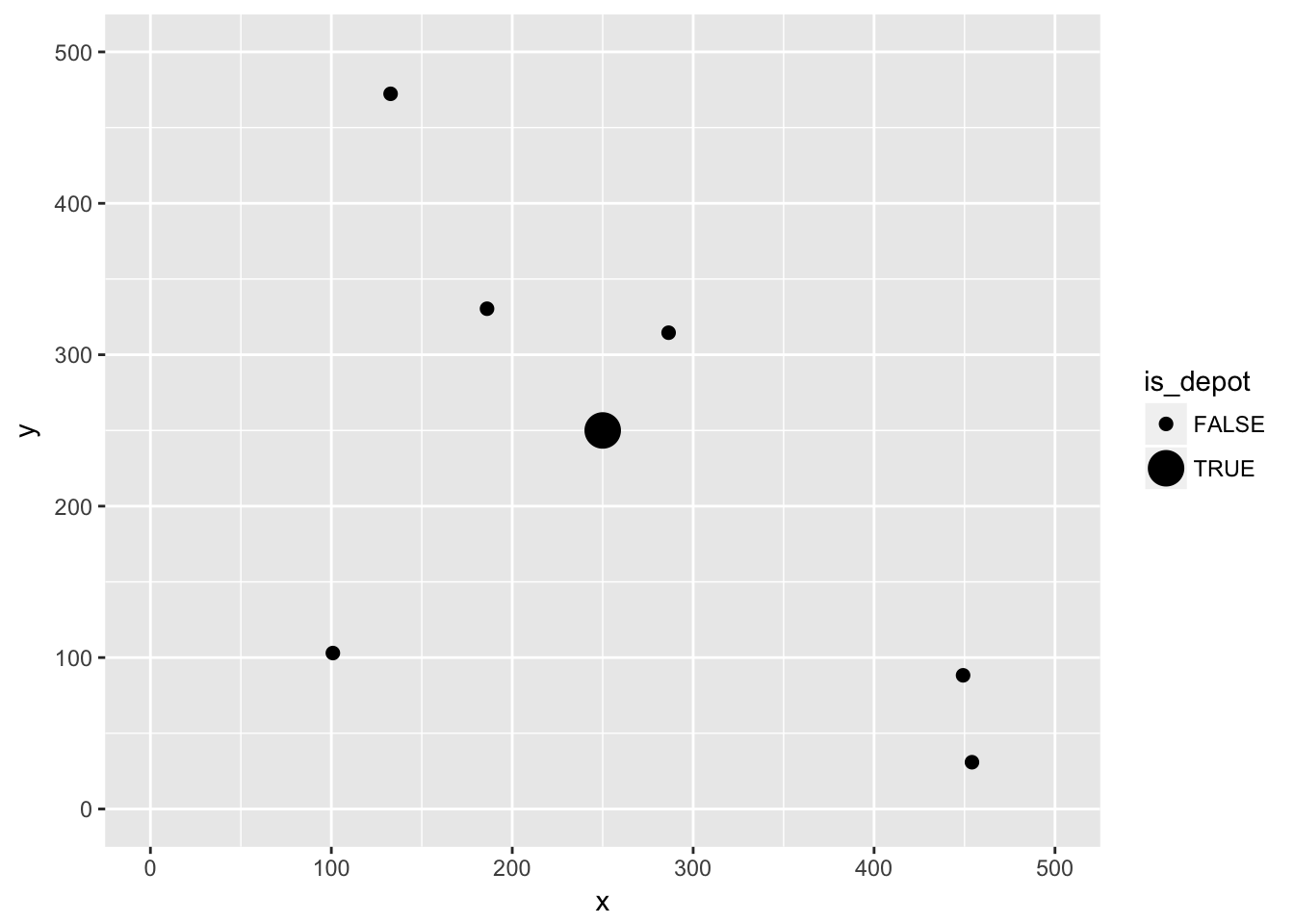

Now the distance matrix

distance <- as.matrix(dist(select(cities, x, y), diag = TRUE, upper = TRUE))

Model formulation

As in the other TSP example we will use the MTZ formulation and solve a fairly small mTSP. The basic idea is to extend the two index formulation to three indexes \(x_{i,j,k}\) that is 1 iff salesman \(k\) travels from \(i\) to \(j\).

Import ompr.

library(ompr)

Formulate the model. By convention the node with index \(1\) is the depot.

# the depot is always idx 1
model <- MIPModel() %>%
  
  # we create a variable that is 1 iff we travel from city i to j by Salesman k
  add_variable(x[i, j, k], i = 1:n, j = 1:n, k = 1:m, type = "binary") %>%
  
  # helper variable for the MTZ sub-tour constraints
  add_variable(u[i, k], i = 1:n, k = 1:m, lb = 1, ub = n) %>% 
  
  # minimize travel distance and latest arrival
  set_objective(sum_expr(distance[i, j] * x[i, j, k], i = 1:n, j = 1:n, k = 1:m), "min") %>%
  
  # you cannot go to the same city
  add_constraint(x[i, i, k] == 0, i = 1:n, k = 1:m) %>%
  
  # each salesman needs to leave the depot
  add_constraint(sum_expr(x[1, j, k], j = 2:n) == 1, k = 1:m) %>%
  
  # each salesman needs to come back to the depot
  add_constraint(sum_expr(x[i, 1, k], i = 2:n) == 1, k = 1:m) %>%
  
  # if a salesman comes to a city he has to leave it as well
  add_constraint(sum_expr(x[j, i, k], j = 1:n) == sum_expr(x[i, j, k], j = 1:n), i = 2:n, k = 1:m) %>%
  
  
  # leave each city with only one salesman
  add_constraint(sum_expr(x[i, j, k], j = 1:n, k = 1:m) == 1, i = 2:n) %>% 
  
  # arrive at each city with only one salesman
  add_constraint(sum_expr(x[i, j, k], i = 1:n, k = 1:m) == 1, j = 2:n) %>% 
  
  # ensure no subtours (arc constraints)
  add_constraint(u[i, k] >= 2, i = 2:n, k = 1:m) %>% 
  add_constraint(u[i, k] - u[j, k] + 1 <= (n - 1) * (1 - x[i, j, k]), i = 2:n, j = 2:n, k = 1:m)
model

## Mixed linear integer optimization problem
## Variables:
##   Continuous: 14 
##   Integer: 0 
##   Binary: 98 
## Search direction: minimize 
## Constraints: 126

Results

This model can now be solved by one of the many solver libraries. Here we will use GLPK.

library(ompr.roi)
library(ROI.plugin.glpk)

result <- solve_model(model, with_ROI(solver = "glpk"))

To extract the solution we can use get_solution method that will return a data.frame which we can further be used with tidyverse packages.

solution <- get_solution(result, x[i, j, k]) %>% 
  filter(value > 0) 
kable(head(solution, 3))

variable	i	j	k	value
x	1	3	2	1
x	1	6	1	1
x	2	4	2	1

Now we need to link back the indexes in our model with the actual cities.

paths <- select(solution, i, j, k) %>% 
  rename(from = i, to = j, salesman = k) %>% 
  mutate(trip_id = row_number()) %>% 
  tidyr::gather(property, idx_val, from:to) %>% 
  mutate(idx_val = as.integer(idx_val)) %>% 
  inner_join(cities, by = c("idx_val" = "id"))
kable(head(arrange(paths, trip_id), 4))

salesman	trip_id	property	idx_val	x	y	is_depot
2	1	from	1	250.0000	250.0000	TRUE
2	1	to	3	186.0619	330.3989	FALSE
1	2	from	1	250.0000	250.0000	TRUE
1	2	to	6	100.8410	102.9873	FALSE

And plot it:

ggplot(cities, aes(x, y)) + 
  geom_point(aes(size = is_depot)) + 
  geom_line(data = paths, aes(group = trip_id, color = factor(salesman))) + 
  ggtitle(paste0("Optimal route with cost: ", round(objective_value(result), 2))) +
  scale_y_continuous(limits = c(0, max_y)) + 
  scale_x_continuous(limits = c(0, max_x))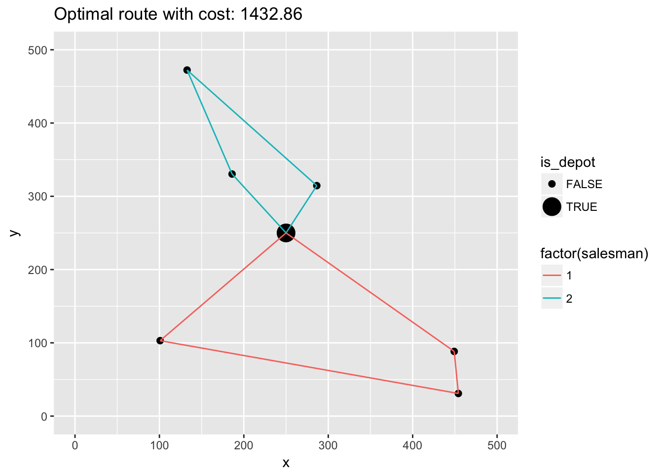

Feedback

Do you have any questions, ideas, comments? Or did you find a mistake? Let’s discuss on Github.