Assigning students to courses

Introduction

In this article we will look at assignment problems.

As a real world example problem we would like to match a group of students to a set of courses with the following constraints:

Each course has a capacity
Every student needs to be assigned to exactly one course.
All students have stated individual preferences on a scale from 1 to 3, where 3 is the most favorable course.

The data

We have \(n\) students:

n <- 40

And \(m\) courses with equal capacity. The capacity can vary among courses though.

m <- 4
capacity <- rep.int(11, m) # all have equal capacities

In addition, each student has three preferences. To model this we have a function that gives us three courses for each student. The first component has perference 1, second 2, and third 3:

set.seed(1234)
preference_data <- lapply(seq_len(n), function(x) sample(seq_len(m), 3))
preferences <- function(student) preference_data[[student]]

preferences(1)

## [1] 4 2 3

The last component we need is a weight functions to make the model formulation easier. This function gives us the preference weighting for a course and student pair.

# the weight of a student choosing a course
# if the course is not among the preferences, the weight is -100000
weight <- function(student, course) {
  p <- which(as.numeric(course) == preferences(as.numeric(student)))
  as.integer(if (length(p) == 0) {
    -100000
  } else {
    p
  })
}

Some examples:

weight(1, 3)

## [1] 3

weight(1, 23) # this was not a choice by student 1, so we give it a big penalty

## [1] -100000

Let’s take a look at our random preferences. We plot the number of votes for each course grouped by the preference (1, 2, 3).

library(ggplot2)
library(purrr)
library(dplyr)
plot_data <- expand.grid(
  course = seq_len(m),
  weight = 1:3
) %>% rowwise() %>% 
  mutate(count = sum(map_int(seq_len(n), ~weight(.x, course) == weight))) %>% 
  mutate(course = factor(course), weight = factor(weight))
ggplot(plot_data, aes(x = course, y = count, fill = weight)) + 
  geom_bar(stat = "identity") + 
  viridis::scale_fill_viridis(discrete = TRUE) + 
  geom_hline(yintercept = 11)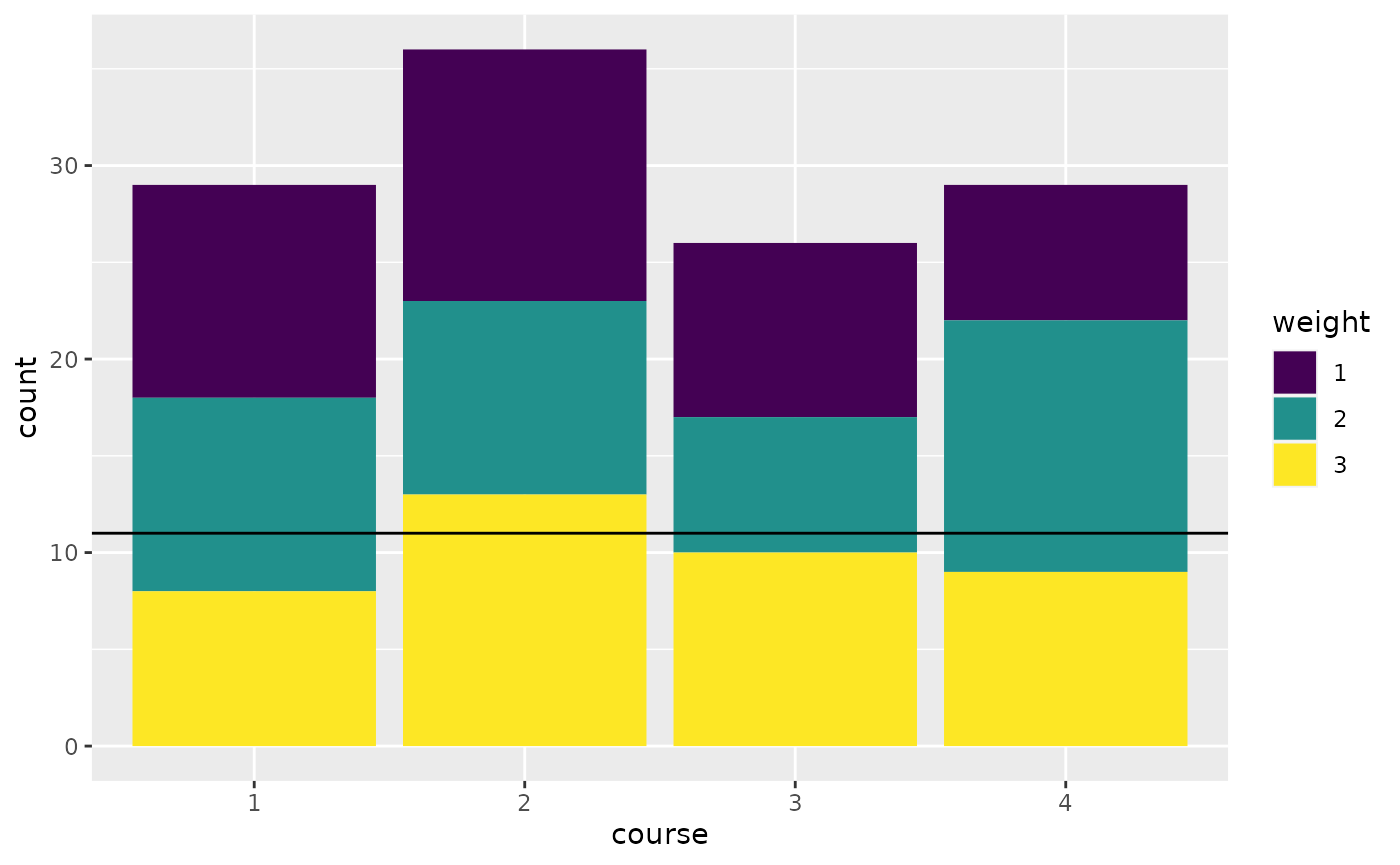

The model

The idea is to introduce a binary variable \(x_{i, j}\) that is \(1\) if student \(i\) is matched to course \(j\). As an objective we will try to satisfy preferences according to their weight. So assigning a student to a course with preference 3 gives 3 points and so forth. The model assumes, that the total capacity of the courses is enough for all students.

Here it is in mathematical notation:

\[ \begin{equation*} \begin{array}{ll@{}ll} \text{max} & \displaystyle\sum\limits_{i=1}^{n}\sum\limits_{j=1}^{m}weight_{i,j} \cdot x_{i, j} & &\\ \text{subject to}& \displaystyle\sum\limits_{i=1}^{n} x_{i, j} \leq capacity_j, & j=1 ,\ldots, m&\\ & \displaystyle\sum\limits_{j=1}^{m} x_{i, j} = 1, & i=1 ,\ldots, n&\\ & x_{i,j} \in \{0,1\}, &i=1 ,\ldots, n, & j=1 ,\ldots, m \end{array} \end{equation*} \]

Or directly in R:

library(ompr)
model <- MIPModel() %>%
  
  # 1 iff student i is assigned to course m
  add_variable(x[i, j], i = 1:n, j = 1:m, type = "binary") %>%
  
  # maximize the preferences
  set_objective(sum_over(weight(i, j) * x[i, j], i = 1:n, j = 1:m)) %>%
  
  # we cannot exceed the capacity of a course
  add_constraint(sum_over(x[i, j], i = 1:n) <= capacity[j], j = 1:m) %>% 
  
  # each student needs to be assigned to one course
  add_constraint(sum_over(x[i, j], j = 1:m) == 1, i = 1:n)
model

## Mixed integer linear optimization problem
## Variables:
##   Continuous: 0 
##   Integer: 0 
##   Binary: 160 
## Model sense: maximize 
## Constraints: 44

Solve the model

We will use glpk to solve the above model.

library(ompr.roi)
library(ROI.plugin.glpk)
result <- solve_model(model, with_ROI(solver = "glpk", verbose = TRUE))

## <SOLVER MSG>  ----
## GLPK Simplex Optimizer 5.0
## 44 rows, 160 columns, 320 non-zeros
##       0: obj =  -0.000000000e+00 inf =   4.000e+01 (40)
##      43: obj =  -8.999410000e+05 inf =   0.000e+00 (0)
## *   140: obj =   1.180000000e+02 inf =   0.000e+00 (0)
## OPTIMAL LP SOLUTION FOUND
## GLPK Integer Optimizer 5.0
## 44 rows, 160 columns, 320 non-zeros
## 160 integer variables, all of which are binary
## Integer optimization begins...
## Long-step dual simplex will be used
## +   140: mip =     not found yet <=              +inf        (1; 0)
## +   140: >>>>>   1.180000000e+02 <=   1.180000000e+02   0.0% (1; 0)
## +   140: mip =   1.180000000e+02 <=     tree is empty   0.0% (0; 1)
## INTEGER OPTIMAL SOLUTION FOUND
## <!SOLVER MSG> ----

We solved the problem with an objective value of 118.

matching <- result %>% 
  get_solution(x[i,j]) %>%
  filter(value > .9) %>%  
  select(i, j) %>% 
  rowwise() %>% 
  mutate(weight = weight(as.numeric(i), as.numeric(j)), 
         preferences = paste0(preferences(as.numeric(i)), collapse = ",")) %>% ungroup

head(matching)

## # A tibble: 6 × 4
##       i     j weight preferences
##   <int> <int>  <int> <chr>      
## 1     4     1      3 4,2,1      
## 2    10     1      3 3,4,1      
## 3    13     1      3 3,4,1      
## 4    15     1      3 4,2,1      
## 5    23     1      3 3,2,1      
## 6    30     1      2 3,1,2

matching %>% 
  group_by(weight) %>% 
  summarise(count = n())

## # A tibble: 2 × 2
##   weight count
##    <int> <int>
## 1      2     2
## 2      3    38

38 students got their top preference. 2 students were assigned to their second choice and 0 students got their least preferable course.

The course assignment now looks like this:

plot_data <- matching %>% 
  mutate(course = factor(j), weight = factor(weight, levels = c(1, 2, 3))) %>% 
  group_by(course, weight) %>% 
  summarise(count = n()) %>% 
  tidyr::complete(weight, fill = list(count = 0))

## `summarise()` has grouped output by 'course'. You can override using the
## `.groups` argument.

ggplot(plot_data, aes(x = course, y = count, fill = weight)) + 
  geom_bar(stat = "identity") + 
  viridis::scale_fill_viridis(discrete = TRUE) + 
  geom_hline(yintercept = 11)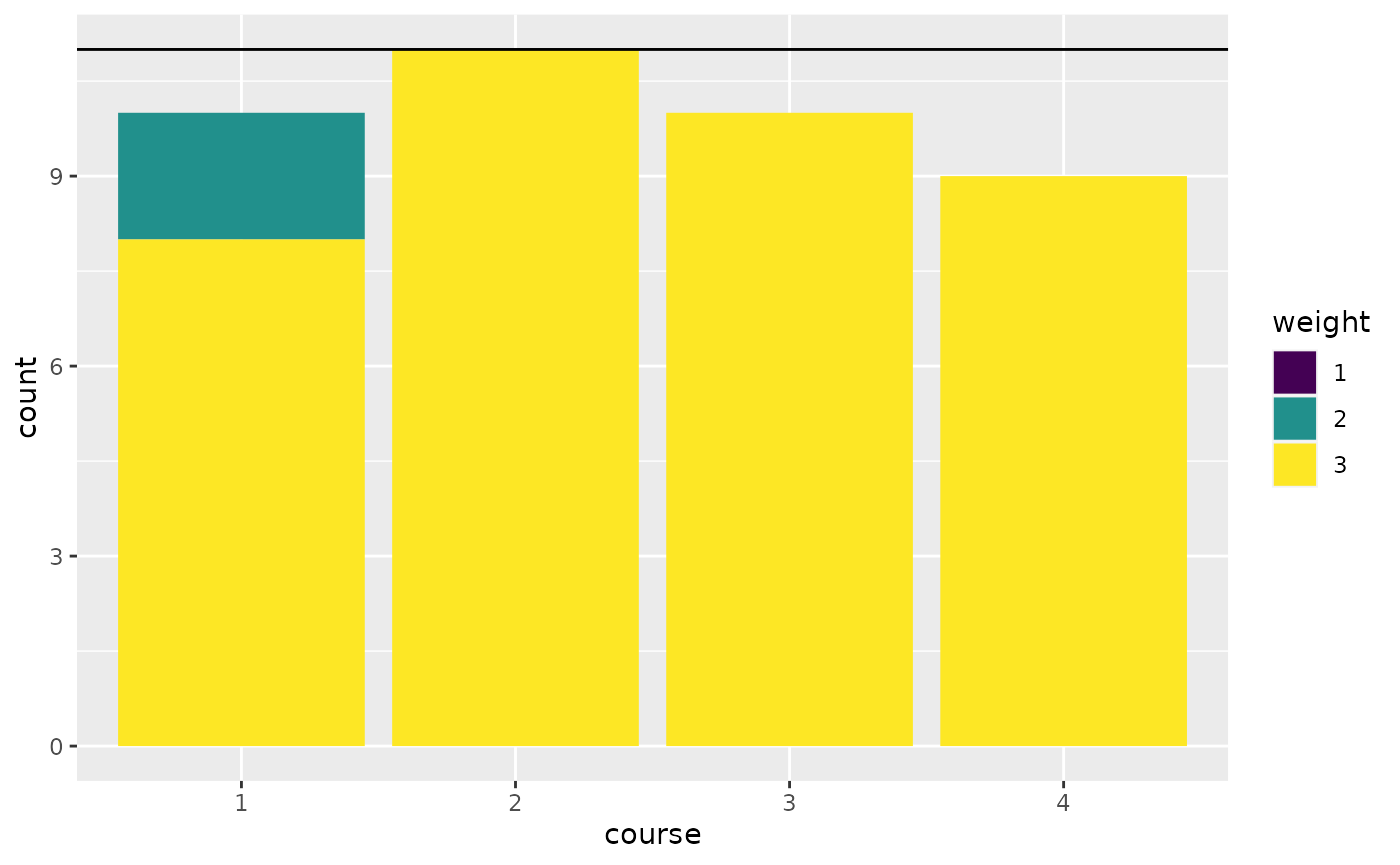

Feedback

Do you have any questions, ideas, comments? Or did you find a mistake? Let’s discuss on Github.

Dirk Schumacher

2016-12-16

Introduction

The data

The model

Solve the model

Feedback